Introduction
The evaluation of large language models has matured considerably in recent years, with benchmarks such as MMLU Hendrycks et al. (2020), GPQA Rein et al. (2023), MATH-Hard Hendrycks et al. (2021), and LiveCodeBench Jain et al. (2024) becoming standard tools for measuring capabilities across scientific knowledge, reasoning, and code generation. These benchmarks have proven effective at differentiating fully trained models, but they share a common blind spot: they were not designed with early training in mind. When applied to small language models (0.5B–3B parameters) during the first 200 billion tokens of training, these benchmarks consistently produce noisy, non-discriminative signals. Scores fluctuate near random baselines, model size orderings break down, and architectural differences become invisible. This is not merely an inconvenience, it represents a fundamental gap in our ability to make informed decisions about hyperparameters, data mixtures, and architectural choices at a stage where such decisions have the greatest downstream impact. The E2LM Competition (Early Training Evaluation of Language Models), hosted at NeurIPS 2025, was designed to address this gap. We provided participants with six pre-trained models across three scales, each with two architectural variants, along with intermediate checkpoints sampled throughout training. The challenge was to design evaluation tasks in the scientific knowledge domain that produce meaningful, monotonically improving signals during early training, while maintaining consistent model rankings at convergence. As a baseline, we demonstrated that even simple prompt reformulations, such as the cloze-style variant of MMLU, can recover informative learning curves where standard multiple-choice formats fail. This observation, inspired by the work of Muennighoff et al. Muennighoff et al. (2024), suggested that the problem lies not in what models know during early training, but in how we ask them to demonstrate it. In this post, we present a retrospective analysis of the competition: we describe the experimental setup proposed to participants, and briefly present the winning solutions.
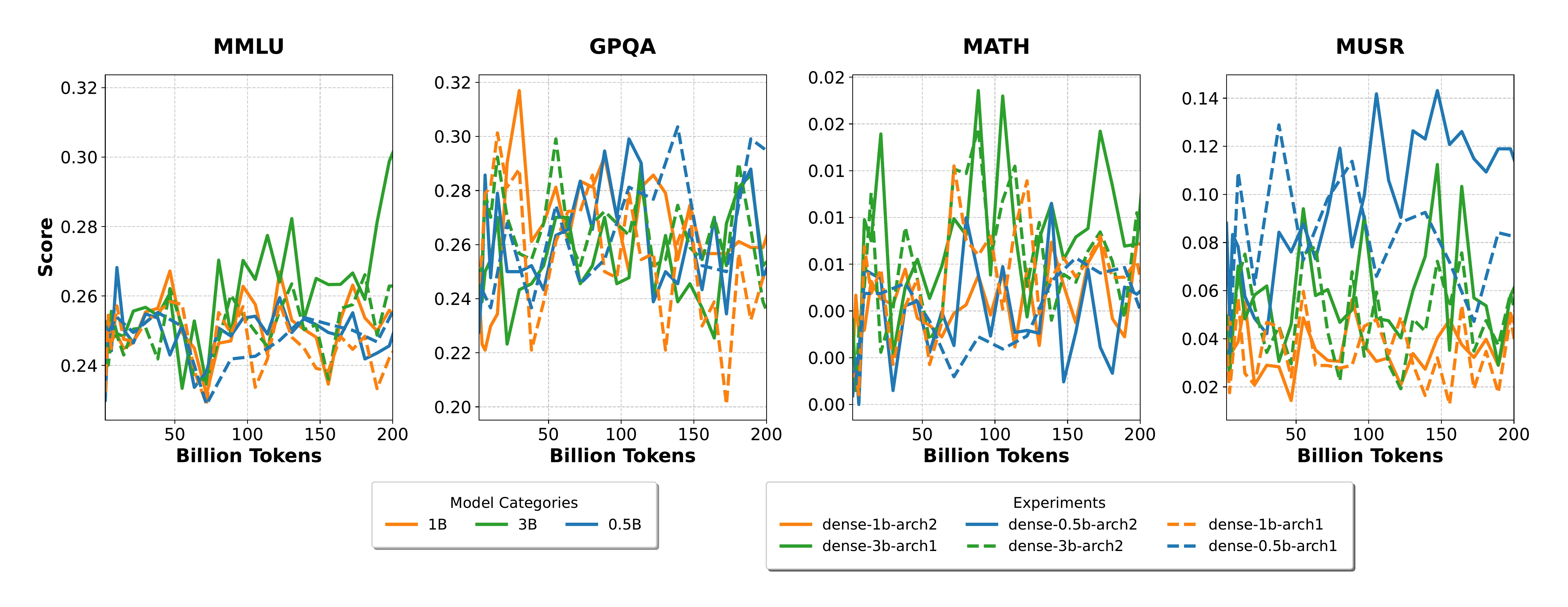
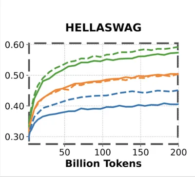
Beyond the noise problem, there is also a question of timing. The earlier we can extract meaningful evaluation signals, the more useful they become. Decisions about data mixtures, architectures, and hyperparameters made in the first few hundred billion tokens have outsized impact on the final model. Yet most scientific benchmarks fail to provide discriminative signals precisely during this critical window, making it costly and difficult to derive conclusive insights from small-scale experiments. This challenge is not uniform across domains. Recent LLM releases have shown rapid improvements on STEM-related tasks such as mathematics and code generation, yet evaluating these capabilities early in training remains particularly difficult. By contrast, commonsense-related benchmarks like HellaSwag Zellers et al. (2019) tend to produce informative signals even at early stages and across model sizes. The gap between what we can measure early (general language understanding) and what we most want to measure early (scientific and reasoning capabilities) is at the heart of this competition. This gap becomes even more pronounced for small language models, which are inherently weaker than their larger counterparts and therefore harder to differentiate using benchmarks designed for frontier models.
MMLU benchmark
Evaluating STEM capabilities of a language model is a topic on its own – MMLU has been proven to be the de facto benchmark to evaluate general scientific knowledge of a language model. MMLU simply consists of MCQ-style questions from various topics, and the target model is prompted to answer a given MCQ question.
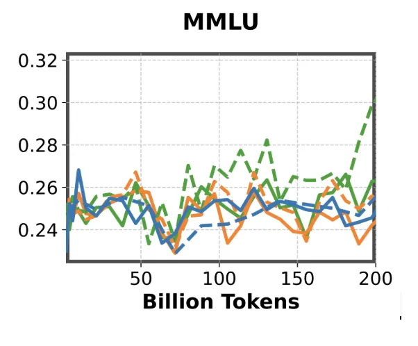
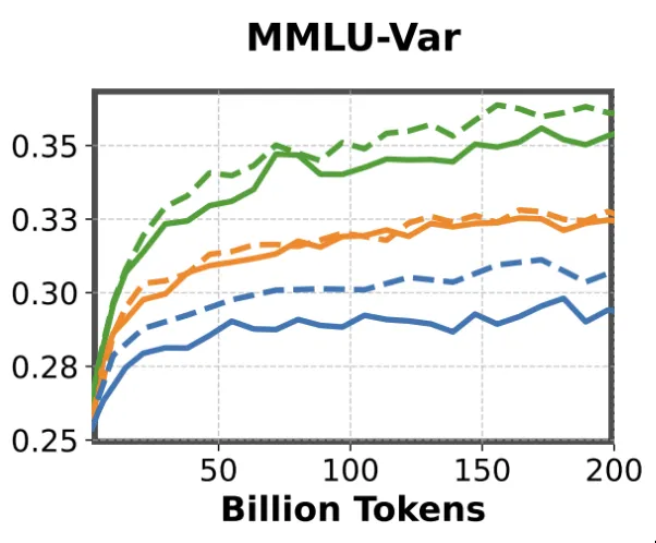
MMLU becomes a meaningful evaluation metric only after a model has been trained on a sufficient number of tokens, and this tends to hold true primarily for models larger than 1B parameters. For smaller models, the benchmark produces essentially random results. Since MMLU is a 4-choice multiple-choice task, a score of around 0.25 corresponds to random guessing, which is often what we observe in these smaller variants. A variant of MMLU, termed as MMLU-Var Muennighoff et al. (2024), is considered today to overcome this problem.
Why MMLU-Var is stable and consistent?
MMLU-Var, a variant of MMLU has been proven to give much stronger signals on Small Language Models. Let’s analyze in detail what is the simple “trick” used by MMLU-Var compared to classic MMLU.
MMLU is a “log-likelihood” style MCQ benchmark. Given a prompt which states the question to be asked to the language model, 4 possible answers are given, and the log-likelihood of the tokens corresponding to the different choices (A, B, C, D) given the question are computed, and an answer is counted as being correct if the highest likelihood corresponds to the actual answer. In this case, as stated above, a random model would give a score of 0.25.
More concretely, assuming we have 4 choices per QA pair, 4 prompts are constructed from the QA pairs with each possible answer.
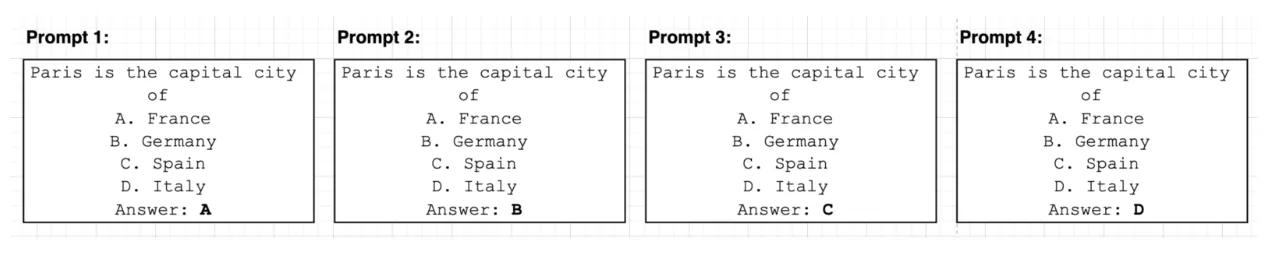
The log-likelihoods are then calculated on the answer tokens, and the answer which has the highest log-likelihood is considered the predicted answer. The answer from the model is then compared against the ground truth answer.
MMLU-Var converts the MCQ format into “completion-mode”. Instead of prompting the model in a MCQ style, 4 different prompts are constructed which represent the continuation version of the MCQ. The log-likelihood is computed on the answer tokens (in case multiple tokens, the sum of the log-likelihoods is considered), and the prompt with the highest log-likelihood on these tokens is considered as the predicted answer from the model.

For small language models, this “trick” converts MMLU benchmark from noisy signals to very meaningful ones. This could be explained by the fact that the trick helps the model to escape from the MCQ domain, which might be hard to grasp during the early training stage of Small Language Models, to a more natural next-token-prediction task.
Why This Matters for the LLM Community?
Given these observations, we believe there is substantial room to explore how existing benchmarks can be adapted to produce higher-quality signals on small language models, and how entirely new evaluation tasks might be designed to capture early training dynamics more effectively. Yet the scope of this problem extends well beyond what any single team can address. Meaningful progress requires the collective engagement of the broader LLM community, drawing on diverse perspectives from machine learning, the domain sciences, and evaluation methodology. This is what motivated us to frame the effort as an open competition. Concretely, we invited participants to investigate several open questions: Can existing popular benchmarks be adapted to yield more meaningful and discriminative signals? Can new benchmarks be designed from the ground up that give informative signal in the early stages of training? Are there alternatives to completion-style prompting that better capture early signals in small language models?
Competition format
The participants were provided multiple model checkpoints to facilitate their benchmark validation. These models were trained on two distinct data mixtures: Web-only data (random subset of FineWeb Penedo et al. (2024), a cleaned, deduplicated English web corpus from CommonCrawl) and Scientific Knowledge Data Mixture (FineWeb-edu Lozhkov et al. (2024) (50%), The Stack V1/V2 Kocetkov et al. (2022) (21.6%), InfiMM Han et al. (2024) (18.9%), TxT360 Tang et al. (2024) (9.5%)). We provided models at three scales each instantiated with two distinct architectural variants for the same size: a deep variant (arch1) and a wide variant (arch2), assuming deeper models reason better (more details can be found in our competition proposal Yagoubi et al. (2025)).
All submissions were independently evaluated across three distinct metrics: Signal Quality (SQ), Ranking Consistency (RC), and Compliance with Scientific Knowledge Domains (CS). The final score was computed as a weighted linear combination of these metrics. Additionally, submissions were validated for alignment with established scientific knowledge domains and screened for potential information leakage.
The overall score was calculated as:
where , , and represent the weight coefficients assigned to each respective metric. These weights were determined based on the relative importance of each evaluation criterion and initialized at , , and , thereby prioritizing signal quality, followed by compliance with scientific knowledge domains, and ranking consistency.
To enable participants to verify the correctness of their approaches locally, participants were provided with a scoring notebook as part of the starter kit, enabling them to compute ScoreSQ using openly available model checkpoints. To mitigate the risk of overfitting to these open checkpoints, a subset of evaluation checkpoints was withheld from participants. Upon submission to the Hugging Face (HF) evaluation space, the overall score was computed automatically using the complete set of checkpoints, and the results were made visible to participants through the platform interface.
Each sub-score offers a concrete metric for assessing whether the benchmark yields meaningful and reliable insights. Broadly, the ScoreSQ component rewards tasks that generate smooth, informative learning curves across the checkpoints, whereas the ScoreRC metric captures the stability, reproducibility, and robustness of model rankings over the full set of checkpoints. Finally, the ScoreCS score evaluates the degree to which the benchmark aligns with principles of sound reasoning and scientific knowledge.
A detailed breakdown of the computation methodologies and evaluation procedures for each sub-score is provided below.
Signal Quality
As mentioned above, this score rewards tasks that produce smooth and informative curves across the evaluated checkpoints. To ensure that only smooth and positive trend curves get rewarded, this score is broken down in two parts:
- Monotonicity Score: To measure the degree of monotonic improvement overtime, we use Spearman’s rank correlation. Given rank differences between iteration indices and their associated scores, the monotonicity score can be computed as:
- Autocorrelation Strength: This component captures temporal coherence where the only signals that are stable over time are rewarded. If we consider an original score sequence and its lagged version (with ) for each lag with . The Pearson’s correlation coefficient between them is calculated as:
The autocorrelation score is the average of the absolute correlations across all lags:
Finally, ScoreSQ can be calculated as the weighted combination of both while weighing both equally so that both directional learning progress as well as temporal stability are rewarded equally.
Ranking Consistency
For the metric to be stable, the ranking of models as training progresses needs to be consistent and reliable, specifically after processing a large number of tokens (1 trillion tokens). Ranking consistency needs to be evaluated for models of different sizes (0.5B, 1B, 3B) separately, and the final score is computed by averaging across these configurations. However, a question arises; how do we measure consistency? Prior works have used Kendall’s Tau Coefficient Kendall (1938) to evaluate the metric consistency across the training steps.
We implemented it as follows:
- Baseline Ranking (at 200 BT): We computed the difference between average performances over 100 and 200 BT for the two architectures (arch1 and arch2) for all model sizes where . The equation is computed as:
where , and and are the scores of models and at checkpoint respectively. If is on average better than , then , otherwise .
- Ranking Consistency Evaluation (between 200 BT and 1TT): Let represent the evaluation points post-200BT. At each point , we compare the current model ranking to the baseline. For each model size , we define
where , and if , otherwise .
Compliance to Reasoning and Knowledge Domains (ScoreCS)
This metric measures whether an evaluation task tests scientific reasoning and knowledge rather than general language or commonsense abilities. From our analysis, science-focused tasks like MMLU-var clearly distinguish between models trained on curated scientific data versus web-only data. By contrast, commonsense benchmarks like HellaSwag produce similar results for both model types, making them unsuitable for this competition.
To quantify domain compliance, we compare two 1B models across training steps: one trained on scientific knowledge data.
This formula normalizes the performance gap, rewarding tasks that effectively measure knowledge-intensive learning regardless of difficulty level.
Metric Scores Analysis
MMLU-var ranks highest overall, followed by ARC-Easy and SciQ, which perform well across all metrics. ARC-Easy is particularly effective for early-stage training assessment and serves as a secondary baseline alongside MMLU-var. However, 82% of SciQ questions contain verbatim answers in their prompts, potentially inflating scores. We address this by applying leakage checks to all submissions and excluding such questions.
Scientific knowledge benchmarks consistently outperform HellaSwag despite its higher Consistency and Signal Quality scores. HellaSwag scores zero on the Compliance metric because it doesn’t test scientific knowledge. While commonsense tasks like HellaSwag and Winogrande appear in our full rankings
To validate our metric’s robustness, similar submissions won’t appear on the official leaderboard as they fail the scientific compliance requirement.
Competition infrastructure
Overall organization
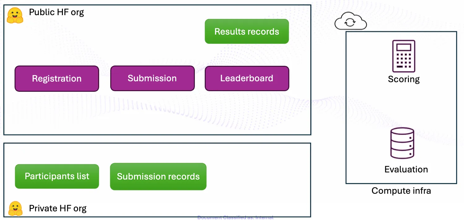
We hosted our competition on a dedicated Hugging Face organization, where teams would join the organization and submit their solutions through a dedicated HuggingFace Space. The submission Space will push each submission bundle in a dedicated private HuggingFace storage. On our side, we fetch the private dataset during each fixed time period and run the series of evaluations. We have also provided the participants various Google Colab notebooks to get started quickly in integrating new benchmarks using the package.
Evaluation backend: lm-evaluation-harness
We asked the participants to develop their benchmarks using lm-evaluation-harness from EleutherAI Gao et al. (2023) - for practical reasons, we have ‘frozen’ the library to a specific commit and made it public under our GitHub organization, and asked the participants to submit git .patch files.
How to submit a benchmark?
Once the benchmark is ready, participants needed to generate the corresponding git .patch file, together with a very simple yaml file that contains few infiormation such as the benchmark name, the metric name as well as an optional HF fine-grained token to eventually access private datasets.
Key Statistics
We present below the key statistics of the competition:
| Metric | Value |
|---|---|
| HF organization members (total participants) | 156 |
| Total submissions | 236 (136 passed, 100 failed) |
| Total registered teams | 128 |
| Total active teams | 12 |
Active teams are defined as those with at least one passed submission. As a side note, we also open source all our models under this Hugging Face collection.
Presentation of Winning solutions
Team Morai
The solution by Team Morai extended the MMLU Var baseline by introducing a novel evaluation metric and a filtering procedure designed to select questions with a meaningful learning signal. Although results are shown on the MMLU benchmark, the team anticipates that these adaptations are applicable to other benchmarks and will yield similar performance improvements.
Proposed metric
Illustrative example with a MCQ in a completion format.
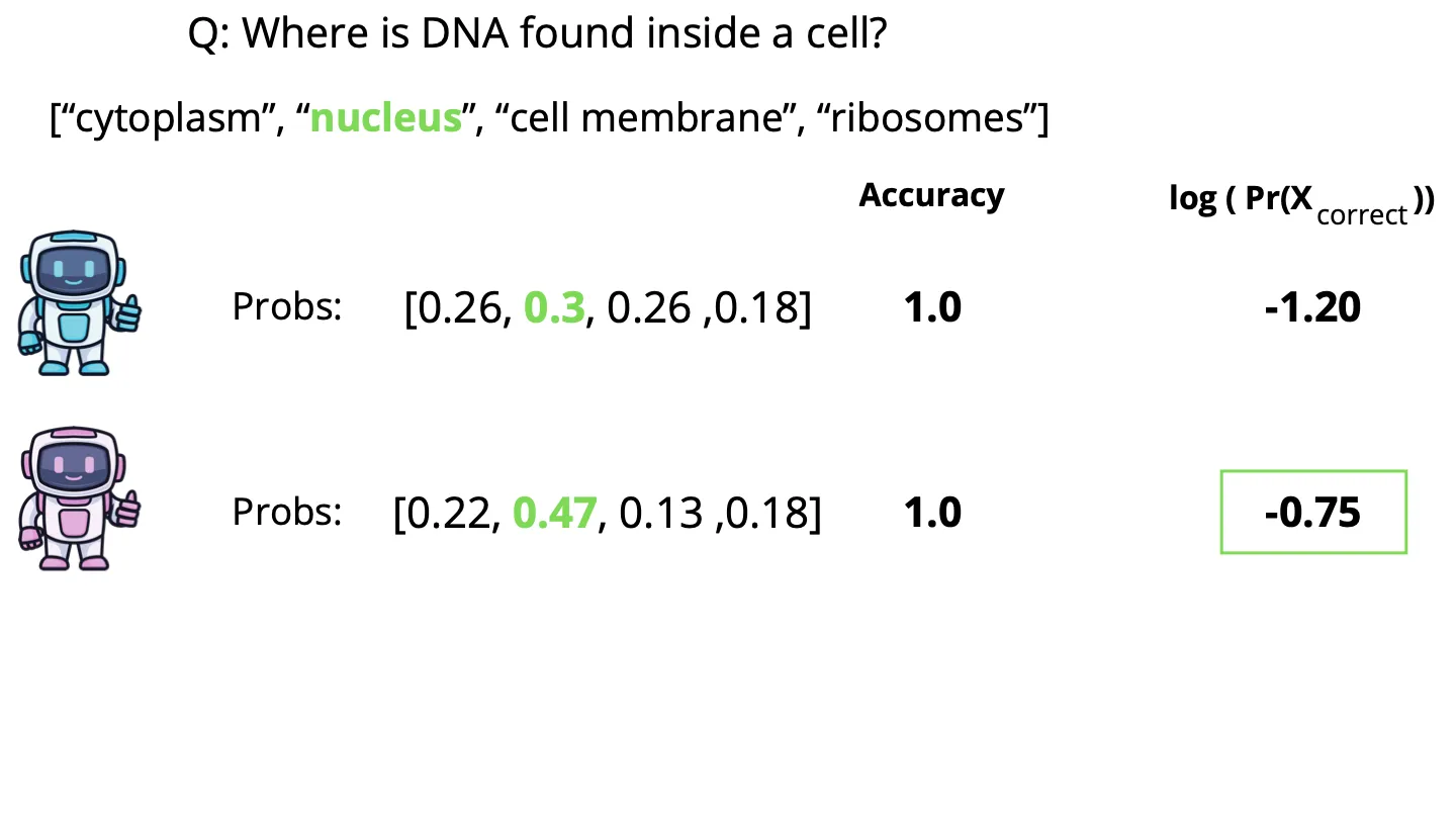
The proposed metric identifies models capable of differentiating between scientific truth and linguistically coherent but factually incorrect text. Although many models demonstrate high linguistic capabilities, that is, generating text that mimics the structure of scientific discourse, the main goal is to select models that prioritize scientific compliance over mere fluency. Given a question , let be the probability assigned by the model to the correct answer, and let be a vector containing the probabilities of the incorrect choices. For example, for a multiple-choice question (MCQ) with four options, has a length of three. Our metric is defined as:
Consider a biology MCQ presented to two models (see Fig. 1). Both models assign the highest probability to the correct answer, resulting in an identical accuracy score of 1. However, since the second model assigns a significantly higher probability to the correct answer, it demonstrates greater “confidence” in the underlying scientific knowledge. A metric defined as the log-likelihood of the correct answer would correctly rank the second model higher.
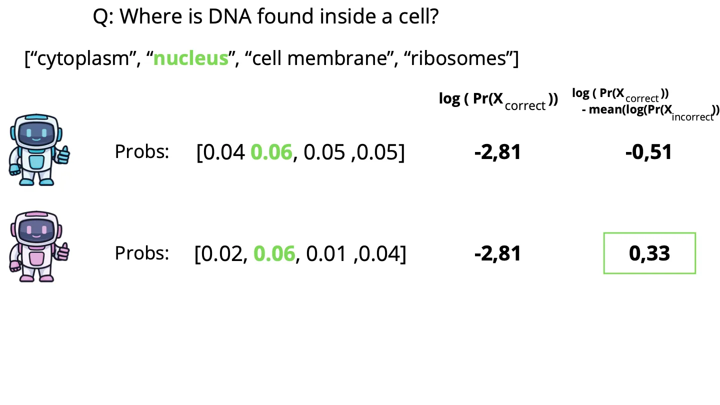
Now, consider a scenario where both models assign an identical probability of 0.6 to the correct answer, as in Fig. 2. A log-likelihood metric would treat them as equivalent. However, if the first model distributes the remaining probability among incorrect answers that are linguistically plausible within the domain, while the second model assigns much lower probabilities to those distractors, the second model exhibits better discriminative power. By applying the metric in Eq. 1, the second model is identified as superior. While alternative formulations, such as omitting the log operator or using operations instead of an average, were considered, preliminary experiments indicated that the current formulation provides the most stable learning signal.
Filtering procedure
Transitioning from a discrete to a continuous metric increases score variance during training. For instance, a model’s probability for a correct answer might shift from 0.06 to 0.062 between checkpoints. While accuracy remains unchanged (both 1), the proposed metrics could increase from 0.33 to 0.35. To distinguish genuine model improvement from random variation, it was implemented a filtering procedure to retain only questions that provide a meaningful learning signal. That is, to exclude those that are either trivial or excessively difficult. Each question in the MMLU dataset was evaluated using the following score:
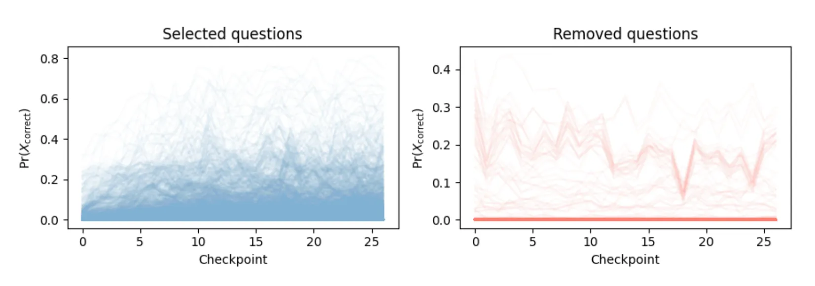
where and represent the probability of the correct answer at the final and initial checkpoints, respectively. A score near 0 indicates a question was either answered correctly from the start (too easy) or remained incorrect throughout training (too hard). This value is averaged across six evaluated architectures. The filtering keep only the top 50% of questions. As shown in Fig. 3, the selected questions predominantly exhibit increasing learning curves. In contrast, the removed questions show a high density at 0, representing items where the model failed to assign any meaningful probability to the correct answer throughout the entire training process.
We compared the proposed metric with and without the filtering procedure. Using the metric alone yielded a global score of 0.72. Implementing the filtering procedure increased this score to 0.801 and significantly improved scientific compliance, which rose from 0.4 to 0.6.
Future directions
The proposed solution still has certain limitations. The current filtering procedure is static, based on initial training iterations. Future work will explore adaptive filtering, where the question subset is updated dynamically as training progresses. Additionally, it was observed a negative correlation between question score and answer length; the filtering approach tends to remove questions with longer textual responses. Future iterations will aim to normalize the methodology to ensure fair evaluation across varying answer lengths.
Team Shaikespear
Introduction
Team Shaikespeare focuses on evaluating a broad range of tasks designed for the challenge. Given the components of the metric used to score the submissions, particular emphasis is placed on scientific compliance. The analysis evaluates the influence of various benchmark characteristics, including the subjects covered by the datasets, individual sample properties, and the evaluation metric itself. The following sections describe the different experiments conducted before reviewing their results. Overall, Team Shaikespeare’s study is organized around three main experiments: (1) evaluating a diverse set of datasets, (2) assessing the performance of a likelihood-based metric, and (3) exploring strategies for filtering large datasets.
Methods
Model prompting
Let denote the parameters of an autoregressive language model defining a distribution over token sequences. For any prompt (context) and continuation , the conditional log-likelihood is
where .
Standard MCQA prompting. In the multiple-choice question answering (MCQA) setting, each instance consists of a question and a finite set of answer candidates , where each is a textual option. A common evaluation protocol formats the input by explicitly enumerating the candidates in the prompt, via a template , and asks the model to output a choice identifier (e.g., a label ). The predicted index is then
This formulation evaluates the model’s ability to discriminate among options when they are jointly presented in-context.
Completion (continuation) mode prompting. Following the competition baseline (MMLU-var), a completion/continuation-based prompting strategy is adopted: the prompt contains the question but omits the answer options, via a template ending with Answer:. Each candidate is then scored as a separate continuation of this prompt, and the selected answer is the one with the highest log-probability under the model. Formally, letting be the tokenization of , we compute
and predict
Datasets
A large range of scientifically oriented datasets was gathered in order to evaluate different dataset characteristics. This corpus comprises existing open datasets as well as a custom one.
Existing Datasets
Most of the datasets used for benchmarking come from publicly released sources. Sub-sampling keeps the number of samples smaller than when source datasets are too large in order to respect the dataset size limitations required by the competition.
- MMLU: Massive Multitask Language Understanding Hendrycks et al. (2020), the original dataset of the competition, used to measure scientific tasks for our LM.
- MMLU Pro: This dataset contains more reasoning-oriented MCQs than the original MMLU Wang et al. (2024).
- OpenBookQA: An MCQ dataset of elementary science understanding and knowledge Mihaylov et al. (2018).
- CS-Bench: A dataset focused on computer science knowledge, including programming, data structures, algorithms, and theoretical concepts. For the team’s benchmark, this dataset was included within the compsci task, where it was merged with computer science-related samples from MMLU and MMLU Pro Song et al. (2025).
- SciKnowEval: A benchmark designed to measure memory, comprehension, reasoning, discernment, and application. The team retained only the memory, comprehension, and reasoning categories Feng et al. (2024).
- TeleQnA: A dataset assessing telecommunications knowledge with question sources including standards and research articles Maatouk et al. (2023).
- MedMCQA: A large-scale medical MCQA dataset of over 190,000 questions from Indian medical entrance exams (AIIMS & NEET PG) that tests clinical knowledge, reasoning, and general medical understanding Pal et al. (2022).
Custom Datasets
To complement the previous benchmarks, the team proposes a novel college-grade dataset comprising MCQA items drawn from course quizzes and exams at Ecole Polytechnique Federale de Lausanne (EPFL). Originally created in 2024 for Direct Preference Optimization (DPO) and Supervised Fine-Tuning (SFT) of large language models, MCQA questions were extracted from these materials to construct the EPFL_QA dataset.
This dataset comprises questions from STEM subjects ranging life science, chemistry, physics, mechanics, computer science, data science, cryptography, math, quantum-physics, machine-learning and information retrieval. Sample QA pairs are given below and show the diversity of questions that evaluate course knowledge or reasoning and may contain numerous symbols.
- Q: The Shannon theorem states that perfect secrecy implies…
C: ['', '', '', ''] - Q: Let be an integer. What is the cardinality of ?
C: '', '', '', '' - Q: To obtain a security of in a hash function against collisions one needs a hash output of size?
C: ’ bits.’, ’ bits.’, ’ bits.’, ’ bits.‘
Metrics
All experiments are conducted using accuracy except when specified otherwise.
Conditional Log-Likelihood (CLL) metric
Because of the binary output of the accuracy metric, non-smooth patterns may appear in the scoring curves, even when large numbers of samples are aggregated. To address this issue, a likelihood-based metric was introduced, the Conditional Log-Likelihood, which computes, given a question/answer pair, the normalized conditional log likelihood of the answer with respect to the question:
where is the question-answer pair and is the probability of the sequence .
Datasets Filtering
Although dataset size influences the scoring metric, large datasets also introduce computational overhead, especially for the competition setup that evaluates submitted tasks once for every model checkpoint.
Three different pruning strategies are presented to keep only the most relevant samples in the current context.
Category based pruning. The team first performs category-based pruning by leveraging the pre-existing partitions provided by the original dataset authors. Concretely, each dataset is partitioned into splits that group samples with shared semantic characteristics. Selected partitions , where , are then evaluated separately.
The team uses this approach to diagnose split-specific contributions to the overall score. In particular, since many datasets are curated with semantically meaningful partitions (e.g., subject areas or skill types), the analysis investigates whether partitions emphasizing science and logic yield higher rewards than others.
Scientific pruning. A scientific score function is defined and used by the team to prune input datasets, retaining only samples that are most intrinsically scientific. This function relies on the previously defined CLL, together with two auxiliary models, and , representing scientific and general-purpose models, respectively. Denoting their corresponding probability density functions as and , the scientific score for a question-answer pair is defined as the difference between the two models’ CLLs:
Samples with higher scores correspond to QA pairs that increase the confidence of the scientific model with respect to the general-purpose one. Because of the scale invariance of this score (doubling both models’ probabilities does not change the score), this function does not discriminate based on sample difficulty and instead evaluates scientific content.
Sample quality pruning. To filter out low-quality web samples, the team uses the GneissWeb data-preparation recipe as implemented in the Data Prep Kit (DPK) (Gohari et al., 2025; Wood et al., 2024). GneissWeb is selected because its recipe is explicitly designed to achieve a favorable quality-quantity trade-off and combines multiple complementary annotators to enable finer-grained filtering decisions.
Concretely, each document (a question-answer pair) is processed in two stages: exact line-level deduplication followed by quality filtering using a combination of learned annotators and heuristic checks. The quality signals computed for each document are described below.
- Document-level quality scores. Two fastText classifiers produce overall quality scores, denoted and .
- Topical category scores. Sentence-level fastText models assign scores for a fixed set of non-exclusive categories . Sentence scores are aggregated to obtain document-level category scores for each .
- Readability score. An inverse readability metric , where lower values indicate better readability.
- Token-per-character ratio. A tokenization-derived statistic used to identify noisy or malformed text:
where is the number of tokenizer output tokens for document .
A document is retained only if it satisfies all of the following conditions:
- Quality gate: it exceeds at least one document-level quality threshold (DCLM or Cosmo).
- Category gates: it exceeds minimum score thresholds for all .
- Readability or tokenization gate: it either has sufficiently good readability or falls within an acceptable range of token-per-character values.
Formally, a document is kept according to the following criterion:
where the thresholds are user defined.
Results
Dataset Analysis of category based pruning
A comparison between STEM and non-STEM oriented datasets is provided in Table 1, which displays the results of the evaluation on different splits of the MMLU and MMLU Pro datasets. These results highlight that technical datasets tend to have better Scientific Compliance (SC).
| Dataset | Signal Quality | Ranking Consistency | Scientific Compliance | Global Score |
|---|---|---|---|---|
| MMLU | 0.959 | 0.837 | 0.419 | 0.731 |
| MMLU STEM | 0.905 | 0.851 | 0.452 | 0.718 |
| MMLU | 0.964 | 0.800 | 0.401 | 0.722 |
| MMLU Pro | 0.928 | 0.730 | 0.542 | 0.754 |
| MMLU Pro STEM | 0.861 | 0.897 | 0.574 | 0.749 |
| MMLU Pro | 0.846 | 0.737 | 0.447 | 0.680 |
Additional evaluations were performed on other datasets and confirm this observation, as seen in Table 2. More verbose datasets tend to have higher Signal Quality (SQ).
| Dataset | Signal Quality | Ranking Consistency | Scientific Compliance | Global Score |
|---|---|---|---|---|
| medmcqa | 0.933 | 0.735 | 0.44 | 0.716 |
| tele_qna | 0.88 | 0.759 | 0.479 | 0.689 |
| compsci | 0.792 | 0.761 | 0.482 | 0.665 |
Influence of the number of tokens per sample
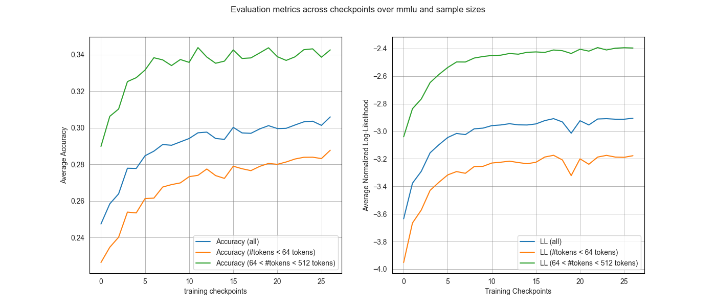
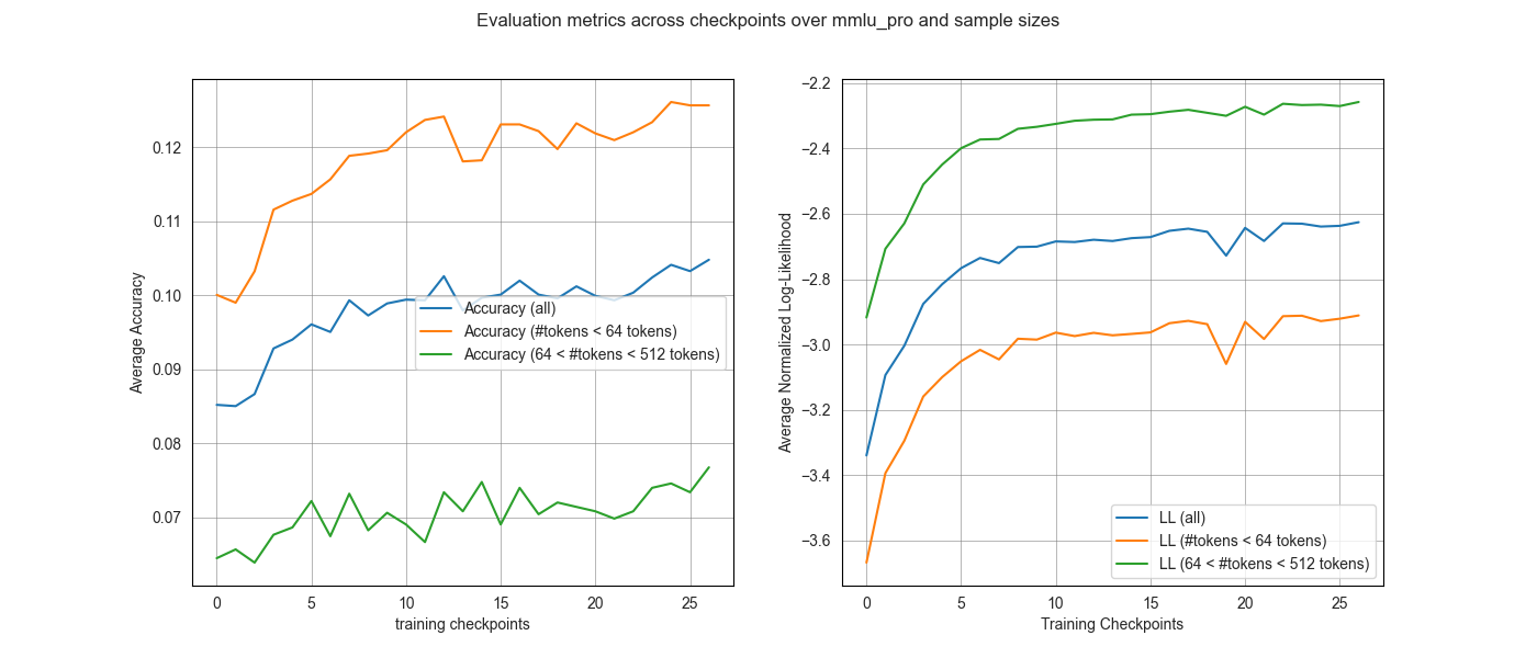
As seen in Figure 1, the number of tokens clearly discriminates the resulting curves, both in terms of accuracy and log-likelihood. One unusual result is how the sample curves corresponding to the higher number of tokens is higher than its counterpart for the MMLU dataset, while it is the opposite for the MMLU Pro dataset, even though both datasets display similar behaviors in log-likelihood.
Notably, the normalized log-likelihood curves exhibit a more consistent ordering across both benchmarks than accuracy does. This suggests that likelihood-based signals (even when normalized) are sensitive to sample length, but provide more stable early-training signals even when accuracy saturates or becomes noisy.
CLL Metric
The CLL metric was compared against the standard accuracy metric on the MMLU Pro dataset, as seen in Table 3, and shows worse scores than the latter, especially for SC.
| Metric | SQ | RC | SC | Score |
|---|---|---|---|---|
| Accuracy | 0.93 | 0.73 | 0.54 | 0.75 |
| CLL | 0.82 | 0.74 | 0.37 | 0.63 |
Custom Dataset: EPFL QA
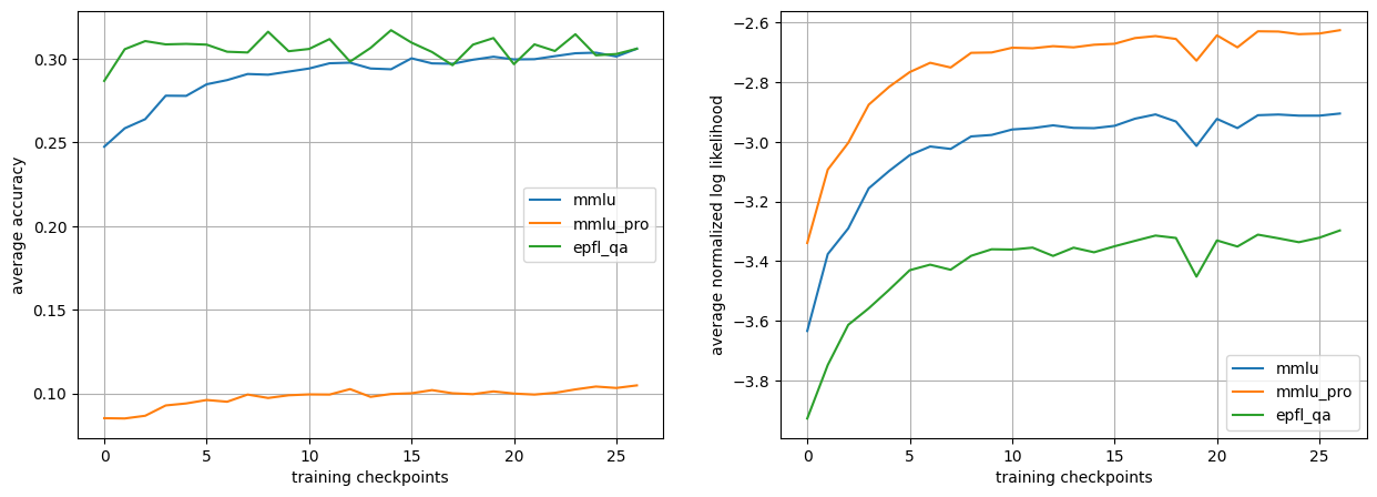
The EPFL_QA dataset resulted in very low scores, seen in Table 5. This is likely due to the fact that many questions in the dataset lack context and may use symbols that are not introduced. In exam settings, the general context information and notations are usually defined once and are not reintroduced in every question.
Another possible reason is the difficulty blend of the dataset, as it contains both easy memorization questions from course quizzes and challenging reasoning and numerical questions. This may explain the early saturation of accuracy, as the model quickly learns how to answer the easy questions, while it never quite succeeds at answering the harder ones, as shown in the left plot of Figure 2. The right sub-figure also motivates this point as it highlights that the average normalized log-likelihood rewards richer and clearer contexts.
Sample quality pruning with GneissWeb
Using the GneissWeb prep kit and starting from the original MMLU collection of MCQA items (each item is a document ), the filtered subsets were constructed
where the team considers the default configuration provided with the recipe, and a strict configuration that tightens multiple filters such that
The metrics on the resulting benchmarks are reported in Table 4.
Overall, the default GneissWeb filtering produces results very similar to the original unfiltered MMLU benchmark. This suggests that moderate pruning can remove low-quality artifacts without changing the benchmark’s underlying signal. By contrast, the strict filtering setting hurts performance: it reduces both ranking consistency and scientific compliance.
To check whether filtering is still keeping the most useful questions, we look at the per-item average score ratio. This ratio captures, on average, how much each remaining item contributes to the total score compared to the unfiltered dataset:
If this ratio is close to 1, filtering kept items that are about as informative as the original average item. If it is much larger than 1, the filtered set is (on average) more informative per question than the original.
| Dataset/Method | SQ | RC | SC | Global Score | Dataset Size | Per Item Avg Score |
|---|---|---|---|---|---|---|
| MMLU | 0.959 | 0.837 | 0.419 | 0.731 | 15858 | 1.00 |
| MMLU + | 0.958 | 0.823 | 0.420 | 0.729 | 14925 | 1.06 |
| MMLU + | 0.956 | 0.737 | 0.396 | 0.710 | 6180 | 2.49 |
Science Score Filtering
The Science score can be used to prune large datasets. Since reasoning-oriented datasets consistently outperform others, as is the case when comparing MMLU Pro to MMLU in Table 1, the choice of auxiliary models can be made in order to retrieve the most reasoning-oriented samples. To this end, the team choose the following two models:
- : LLaMA 3.2 1B-Instruct (general model)
- : LogiLLaMA (reasoning model), an instance of the previous model fine-tuned on scientific reasoning data.
This filtering was performed to keep only samples out of a dataset merging MMLU, MMLU Pro, and EPFL_QA. Subsequent results are shown in Table 5 with the SciScore pruning entry.
General Results
The general results in Table 5 crown the SciKnowEval benchmark. It is still worth mentioning that there is no clear winner in all categories.
| Dataset/Method | Signal Quality | Ranking Consistency | Scientific Compliance | Global Score |
|---|---|---|---|---|
| EPFL_QA | 0.40 | 0.72 | 0.19 | 0.35 |
| MMLU Pro (CLL) | 0.82 | 0.74 | 0.37 | 0.63 |
| openbook_qa | 0.87 | 0.85 | 0.35 | 0.66 |
| compsci | 0.79 | 0.76 | 0.48 | 0.66 |
| tele_qna | 0.88 | 0.76 | 0.48 | 0.69 |
| medmcqa | 0.93 | 0.73 | 0.44 | 0.72 |
| SciScore pruning | 0.90 | 0.81 | 0.47 | 0.72 |
| MMLU | 0.96 | 0.84 | 0.42 | 0.73 |
| MMLU Pro | 0.93 | 0.73 | 0.54 | 0.75 |
| SciKnowEval | 0.93 | 0.75 | 0.55 | 0.76 |
Conclusion and Perspectives
This work investigates early-stage evaluation and data curation strategies for scientific and logic-oriented language model training. The team’s results indicate that reasoning-focused datasets consistently improve scientific compliance, suggesting that the nature of the training signal matters already in the early regime. At the same time, the team deduced that likelihood-based metrics on their own do not reliably capture the behaviors of interest, and can be confounded by surface-form properties. In addition, sample length and verbosity substantially influence early signals, which motivates controlling for these factors when designing new benchmarks for early evaluation.
Looking ahead, an important direction is to incorporate explicit notions of sample difficulty into both pruning procedures and likelihood-based evaluation, so that filtering and scoring account for more than fluency and format effects. In parallel, benchmark design should better balance two competing objectives: producing smooth, stable curves at early checkpoints while still discriminating meaningfully between scientific reasoning capabilities. Together, these directions may lead to more faithful early proxies for downstream scientific performance and more effective data selection policies.
Team Noor
Evaluating Large Language Models (LLMs) at early stages of training remains a significant challenge. During this phase, models exhibit unstable behavior, and traditional metrics such as accuracy often produce noisy and volatile signals that obscure genuine learning progress. As a result, it becomes difficult to distinguish meaningful improvements from random fluctuations.
Rather than generating synthetic evaluation data, the team focuses on extracting a high-quality, high-signal subset from the existing MMLU-var benchmark. The analysis argues that many challenges associated with early-stage evaluation arise not from the models themselves, but from the inclusion of questions that either lack strong scientific grounding or fail to reflect progressive learning.
The objective is therefore twofold: (i) ensuring strict scientific relevance, and (ii) maximizing signal quality, defined as the smoothness and monotonicity of learning trajectories across training checkpoints.
Methodology
To enable rapid experimentation while remaining compute-efficient, the team adopted a compute once, filter many times strategy. All evaluation signals are precomputed in a single pass, enabling iteration exclusively on filtering logic without re-running expensive model evaluations.
1 - Comprehensive Data Generation
The team evaluated all three competition models (Dense-500M, Dense-1B, and Dense-3B) across all provided training checkpoints on the full MMLU-var dataset. For each question, the log-likelihood of all answer choices was computed, and the most probable option was selected as the model’s prediction. In addition to binary accuracy, the full log-probability distribution over choices was stored, enabling the computation of confidence-based metrics. This process resulted in a dense performance database containing accuracy and fine-grained confidence signals for every question-model-checkpoint triplet.
2 - Filtering Pipeline
From this comprehensive dataset, the team applied a two-stage filtering pipeline designed to retain only questions that are both scientifically grounded and informative of learning progress.
Scientific Compliance
The first stage enforces strict scientific relevance. Core Hard Science subjects, such as Mathematics, Physics, and Electrical Engineering, were automatically retained due to their well-defined and technical nature. For other scientific domains, including Biology, Medicine, and Computer Security, a rigorous validation step was applied using a Qwen2.5-7B LLM judge. Each question was independently prompted five times, and only those receiving a unanimous Accept verdict were retained. This strict criterion prioritizes precision over coverage, ensuring high scientific alignment.
Signal Quality Optimization
The second stage targets the quality of the learning signal. For each remaining question, the evolution of a confidence-based score across training checkpoints was tracked and fit a linear regression line to this trajectory. Only questions exhibiting a positive slope—indicating consistent improvement over time—were retained. This step removes questions that are noisy, stagnant, or uninformative despite being scientifically valid.
Evaluation Metric: Confidence Margin
A central finding of the team’s work is the superiority of the Confidence Margin over standard accuracy for early-stage large language model evaluation. The Confidence Margin is defined as:
This metric captures not only whether the model selects the correct answer, but also how strongly it prefers it relative to the most competitive distractor.
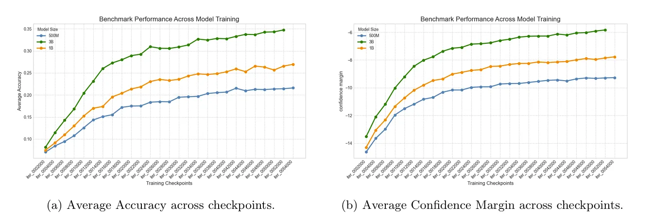
Empirically, it is observed that accuracy curves at early checkpoints are highly volatile and non-monotonic, whereas Confidence Margin trajectories are significantly smoother. This allows the metric to reveal gradual learning dynamics that accuracy fails to capture, such as the steady promotion of the correct answer within the probability ranking before it becomes the top choice.
Conclusion
By combining a strict scientific compliance filter with a signal-quality filter based on Confidence Margin regression, the team constructed a benchmark that offers a clearer and more reliable lens for observing early-stage LLM development. The results suggest that improving early-stage evaluation does not necessarily require new data, but rather careful curation of existing benchmarks guided by metrics that reflect learning dynamics instead of final correctness alone.
Perspectives and Future Work
This work opens several promising directions for future research. First, signal modeling could be extended beyond linear trends to capture more complex learning dynamics. Second, subject-aware filtering strategies could account for differing learning behaviors across scientific domains. Finally, the proposed pipeline is benchmark-agnostic and could be applied to other evaluation datasets, contributing to more interpretable and reliable assessment of emerging LLMs.
Integration within lm-evaluation-harness
For winning solutions, we have decided to offer a native integration with the popular lm-evaluation-harness package in collaboration with the library authors and the participants.
Anyone can use easily the benchmarks developed by the winning solutions starting from now, by making sure to install the latest version of lm-eval: pip install -U lm_eval. Below is an example command you can refer to:
lm_eval --model hf \
  --model_args pretrained=tiiuae/Falcon-H1-0.5B-Base \
  --tasks mmlu_early_training \ # `sciknoweval_mcqa` or `noor`
  --device cuda:0 \
  --batch_size auto
Discussion
The E2LM competition asked whether we can design evaluation tasks that produce useful signals during early training. The results suggest that the challenge is twofold: it involves both what we evaluate and how we evaluate it. On one hand, prompt format plays a critical role: standard multiple-choice formats fail not because early-stage models lack scientific understanding, but because the format requires capabilities, such as comparing and choosing between options, that only develop later in training. On the other hand, the content and difficulty of the questions themselves matter just as much: benchmarks that are too hard, too easy, or poorly calibrated for the model’s developmental stage produce uninformative signals regardless of how they are prompted. Beyond prompt format, the competition highlighted several complementary strategies. Confidence-based metrics such as the Confidence Margin and log-probability gap consistently performed better than raw accuracy at detecting gradual learning progress. Careful selection of evaluation samples, through learning-curve-based filtering, scientific compliance scoring, or data quality pruning, can meaningfully improve benchmark quality without the need to create new data. Participants also went beyond adapting existing benchmarks: the EPFL_QA dataset, built from university-level STEM exams, represents a notable effort to create an entirely new evaluation resource from scratch. Building such a benchmark is far from straightforward: it requires collecting domain-specific content, calibrating difficulty appropriately, and handling challenges specific to academic material such as implicit context and notation. While the initial results exposed these difficulties, the dataset itself provides a solid starting point that the community can improve, expand, and adapt to other scientific fields.
What’s Next?
The E2LM competition has opened several promising research directions that we believe deserve continued attention from the community:
Building new evaluation resources The EPFL_QA dataset demonstrated both the value and the difficulty of creating benchmarks from scratch. While university-level exams are a natural source of calibrated scientific questions, adapting them for LLM evaluation requires careful handling of implicit context, notation, and difficulty distribution. We believe that extending it to other disciplines could yield a rich and diverse evaluation ecosystem for early training.
From early signals to scaling predictions. Our results offer encouraging evidence that early evaluation can serve as a reliable proxy for later training behavior: for benchmarks like MMLU-var and ARC-Easy, model rankings established at 200 billion tokens remained largely consistent through 1 trillion tokens. However, this consistency was not uniform across all configurations, and it remains to be seen whether these findings generalize beyond the 3B scale. Establishing a formal connection between early-stage signals and final model capabilities would be a significant step — it would allow practitioners to make confident architectural and data decisions based on a fraction of the total training compute.
Extending beyond scientific knowledge. This competition focused specifically on the scientific knowledge domain, but the underlying challenge (extracting meaningful evaluation signals during early training) applies broadly. Code generation, mathematical reasoning, and multilingual capabilities all face similar issues with noisy early benchmarks. Adapting the strategies and metrics explored here to these domains is a natural extension of this work.
Authors
| Team | Authors |
|---|---|
| FalconLLM | Younes Belkada, Mugariya Farooq, Basma Boussaha, Mouadh Yagoubi, Yasser Dahou, Phuc Le Khac, Billel Mokeddem, Reda Alami |
| Shaikespear | Anthony Kalaydjian, Eric Saikali |
| Morai | Beatriz Nascimento, Daniel Gardin, Caio Rhoden, Giovani Valdrighi |
| Noor | Mohammed Dahbani, Anas Ezzakri |
| EleutherAI | Baber Abbasi |
- Feng, K., Ding, K., Wang, W., Zhuang, X., Wang, Z., Qin, M., Zhao, Y., Yao, J., Zhang, Q., & Chen, H. (2024). Sciknoweval: Evaluating multi-level scientific knowledge of large language models. arXiv Preprint arXiv:2406.09098.
- Gao, L., Tow, J., Abbasi, B., Biderman, S., Black, S., DiPofi, A., Foster, C., Golding, L., Hsu, J., Le Noac’h, A., Li, H., McDonell, K., Muennighoff, N., Ociepa, C., Phang, J., Reynolds, L., Schoelkopf, H., Skowron, A., Sutawika, L., … Zou, A. (2023). A framework for few-shot language model evaluation (v0.4.0). Zenodo. 10.5281/zenodo.10256836
- Gohari, H. E., Kadhe, S. R., Shah, S. Y., Adam, C., Adebayo, A., Adusumilli, P., Ahmed, F., Angel, N. B., Borse, S., Chang, Y.-C., Dang, X.-H., Desai, N., Eres, R., Iwamoto, R., Karve, A., Koyfman, Y., Lee, W.-H., Liu, C., Lublinsky, B., … Bhattacharjee, B. (2025). GneissWeb: Preparing High Quality Data for LLMs at Scale. https://arxiv.org/abs/2502.14907
- Han, X., Jian, Y., Hu, X., Liu, H., Wang, Y., Fan, Q., Ai, Y., Huang, H., He, R., Yang, Z., & You, Q. (2024). InfiMM-WebMath-40B: Advancing Multimodal Pre-Training for Enhanced Mathematical Reasoning. https://arxiv.org/abs/2409.12568
- Hendrycks, D., Burns, C., Basart, S., Zou, A., Mazeika, M., Song, D., & Steinhardt, J. (2020). Measuring massive multitask language understanding. arXiv Preprint arXiv:2009.03300. back: 1, 2
- Hendrycks, D., Burns, C., Kadavath, S., Arora, A., Basart, S., Tang, E., Song, D., & Steinhardt, J. (2021). Measuring Mathematical Problem Solving With the MATH Dataset. arXiv Preprint arXiv:2103.03874.
- Jain, N., Han, K., Gu, A., Li, W.-D., Yan, F., Zhang, T., Wang, S., Solar-Lezama, A., Sen, K., & Stoica, I. (2024). LiveCodeBench: Holistic and Contamination Free Evaluation of Large Language Models for Code. https://arxiv.org/abs/2403.07974
- Kendall, M. G. (1938). A New Measure of Rank Correlation. Biometrika, 30(1–2), 81–93. 10.1093/biomet/30.1-2.81
- Kocetkov, D., Li, R., Ben Allal, L., Li, J., Mou, C., Muñoz Ferrandis, C., Jernite, Y., Mitchell, M., Hughes, S., Wolf, T., Bahdanau, D., von Werra, L., & de Vries, H. (2022). The Stack: 3 TB of permissively licensed source code. Preprint.
- Lozhkov, A., Ben Allal, L., von Werra, L., & Wolf, T. (2024). FineWeb-Edu: the Finest Collection of Educational Content . Hugging Face . https://doi.org/ 10.57967/hf/2497
- Maatouk, A., Ayed, F., Piovesan, N., Domenico, A. D., Debbah, M., & Luo, Z.-Q. (2023). TeleQnA: A Benchmark Dataset to Assess Large Language Models Telecommunications Knowledge. https://arxiv.org/abs/2310.15051
- Mihaylov, T., Clark, P., Khot, T., & Sabharwal, A. (2018). Can a suit of armor conduct electricity? a new dataset for open book question answering. arXiv Preprint arXiv:1809.02789.
- Muennighoff, N., Soldaini, L., Groeneveld, D., Lo, K., Morrison, J., Min, S., Shi, W., Walsh, P., Tafjord, O., Lambert, N., & others. (2024). Olmoe: Open mixture-of-experts language models. arXiv Preprint arXiv:2409.02060. back: 1, 2
- Pal, A., Umapathi, L. K., & Sankarasubbu, M. (2022). Medmcqa: A large-scale multi-subject multi-choice dataset for medical domain question answering. Conference on Health, Inference, and Learning, 248–260.
- Penedo, G., Kydlíček, H., allal, L. B., Lozhkov, A., Mitchell, M., Raffel, C., Werra, L. V., & Wolf, T. (2024). The FineWeb Datasets: Decanting the Web for the Finest Text Data at Scale. https://arxiv.org/abs/2406.17557
- Rein, D., Hou, B. L., Stickland, A. C., Petty, J., Pang, R. Y., Dirani, J., Michael, J., & Bowman, S. R. (2023). GPQA: A Graduate-Level Google-Proof Q&A Benchmark. https://arxiv.org/abs/2311.12022
- Song, X., Diao, M., Dong, G., Wang, Z., Fu, Y., Qiao, R., Wang, Z., Fu, D., Wu, H., Liang, B., Zeng, W., Wang, Y., GongQue, Z., Yu, J., Tan, Q., & Xu, W. (2025). CS-Bench: A Comprehensive Benchmark for Large Language Models towards Computer Science Mastery. https://arxiv.org/abs/2406.08587
- Tang, L., Ranjan, N., Pangarkar, O., Liang, X., Wang, Z., An, L., Rao, B., Jin, L., Wang, H., Cheng, Z., Sun, S., Mu, C., Miller, V., Ma, X., Peng, Y., Liu, Z., & Xing, E. P. (2024). TxT360: A Top-Quality LLM Pre-training Dataset Requires the Perfect Blend.
- Wang, Y., Ma, X., Zhang, G., Ni, Y., Chandra, A., Guo, S., Ren, W., Arulraj, A., He, X., Jiang, Z., Li, T., Ku, M., Wang, K., Zhuang, A., Fan, R., Yue, X., & Chen, W. (2024). MMLU-Pro: A More Robust and Challenging Multi-Task Language Understanding Benchmark. https://arxiv.org/abs/2406.01574
- Wood, D., Lublinsky, B., Roytman, A., Singh, S., Adam, C., Adebayo, A., An, S., Chang, Y. C., Dang, X.-H., Desai, N., Dolfi, M., Emami-Gohari, H., Eres, R., Goto, T., Joshi, D., Koyfman, Y., Nassar, M., Patel, H., Selvam, P., … Daijavad, S. (2024). Data-Prep-Kit: getting your data ready for LLM application development. https://arxiv.org/abs/2409.18164
- Yagoubi, M., Dahou, Y., Mokeddem, B., Belkada, Y., Le-Khac, P. H., Boussaha, B. E. A., Alami, R., Zuo, J., Marsili, D., Farooq, M., Lalmas, M., Gkioxari, G., Gallinari, P., Torr, P., & Hacid, H. (2025). NeurIPS 2025 E2LM Competition: Early Training Evaluation of Language Models. https://arxiv.org/abs/2506.07731
- Zellers, R., Holtzman, A., Bisk, Y., Farhadi, A., & Choi, Y. (2019). HellaSwag: Can a Machine Really Finish Your Sentence? https://arxiv.org/abs/1905.07830